LISA Data Challenge 2a new generation: Sangria-HM, more fruity, better taste
We are pleased to announce the release of the Sangria-HM dataset. This new dataset contains exactly the same sources as the original Sangria data, but we have used a different GW model for MBHBs. The model is based on the PhenomHM and its implementation in the lisabeta package. The waveform is generated in the frequency domain for (2,2), (2,1), (3,3), (3,2), (4,3) and (4,4) harmonics (amplitude and phase). The GW strain (two polarisations, h+ and hx) are constructed in the time domain by summing up harmonics. Each harmonic was transformed to the time domain by inverse Fourier transform (np.fft.irfft) of the windowed merger part and using stationary phase approximation for the inspiral. Both parts are stitched together in the time domain in the common region of validity.
The instrumental noise was regenerated using the same (as in Sangria) spectral shape.
The aim of this dataset:
- Inclusion of the higher modes should reduce the degeneracies in the MBHB parameter recovery.
- A different noise realisation might tell us more about the bias that we observed for source #10 in Sangria results.
- This data set can be used in low-latency investigations as it is more appropriate for the source localisation in the sky.
Analyse the data and submit it in the same format as for Sangria.
LISA Data Challenge 2a: Sangria
We are glad to announce the release of the first two datasets in the second LISA Data Challenge, codenamed Sangria.
The purpose of this challenge is to tackle mild source confusion with idealized instrumental noise. Datasets mixing different types of GW sources are also referred to as "enchiladas". If you are new to the Challenges, we strongly advise that you first complete the first data challenge Radler before moving to Sangria, and specifically the full Galaxy (LDC1-4 v2) and single massive black-hole binary (LDC1-1 v2) datasets. The first data challenge is officially closed, but we will acknowledge your submission and include it in the evaluation of solutions.
Sangria includes two main datasets: each contains Gaussian instrumental noise and simulated waveforms from 30 million Galactic white dwarf binaries, from 17 verification Galactic binaries, and from merging massive black-hole binaries with parameters derived from an astrophysical model. The first dataset includes the full specification used to generate it: source parameters, a description of instrumental noise with the corresponding power spectral density, LISA's orbit, etc. We also release noiseless data for each type of source, for waveform validation purposes. The second dataset is blinded: the level of istrumental noise and number of sources of each type are not disclosed (except for the known parameters of the verification binaries).
The datasets were generated with a new process meant to prototype the large-scale simulations that will be needed in the LISA science ground segment. For each source we produced time series of the two gravitational-wave polarizations, and projected them onto the LISA laser links. The sum of all projections was ran through LISACode to produce "TDI-1.5" observables X, Y, Z, expressed as fractional frequency corrections, downsampled to 5-second cadence. The datasets cover 1 year: you are welcome to analyze them in full, or in segments of increasing length, reproducing the realistic case where data is progressively downlinked from the spacecraft.
The code and pipeline used to generate the datasets are released as the first version of the new LDC toolbox, accessible in the LISA Consortium GitLab. This Python toolbox will be the foundation for a set of LISA common tools, to be used to generate and analyze the data (including physical constants, orbits, I/O utilities, waveform generation, noise characterization, and so on). The data-generation pipeline is built on top of the toolbox, using the Snakemake workflow manager to orchestrate the multiple steps needed to build the dataset. Documentation is provided so that anyone may reproduce the dataset, or generate custom datasets for other studies. Notebook tutorials are also provided to help gain familiarity with the LDC toolbox and data format.
LDC working-group members will be preparing their own analysis using their algorithms of choice, and invite you to join them (to do so, e-mail us so we can pair you appropriately). Of course, you may organize to work on your own, or with your collaborators. For usage tracking purposes, we request that you set up a login for this website before downloading the datasets (your LDC-1 login will work fine). Please submit your results by October 1st, 2021, using the submission interface and format to be found on this website. Plan to include a description of your methods (or a link to a methods paper) with your submission. We would also greatly appreciate it if you were to share your code (e.g., on GitHub, or on our GitLab).
While we did our best to check the datasets for correctness, small problems or inconsistencies may have escaped us. The best way to validate the data is to analyze it, so let us know of any problems!
LDC2a-v1. Training dataset.
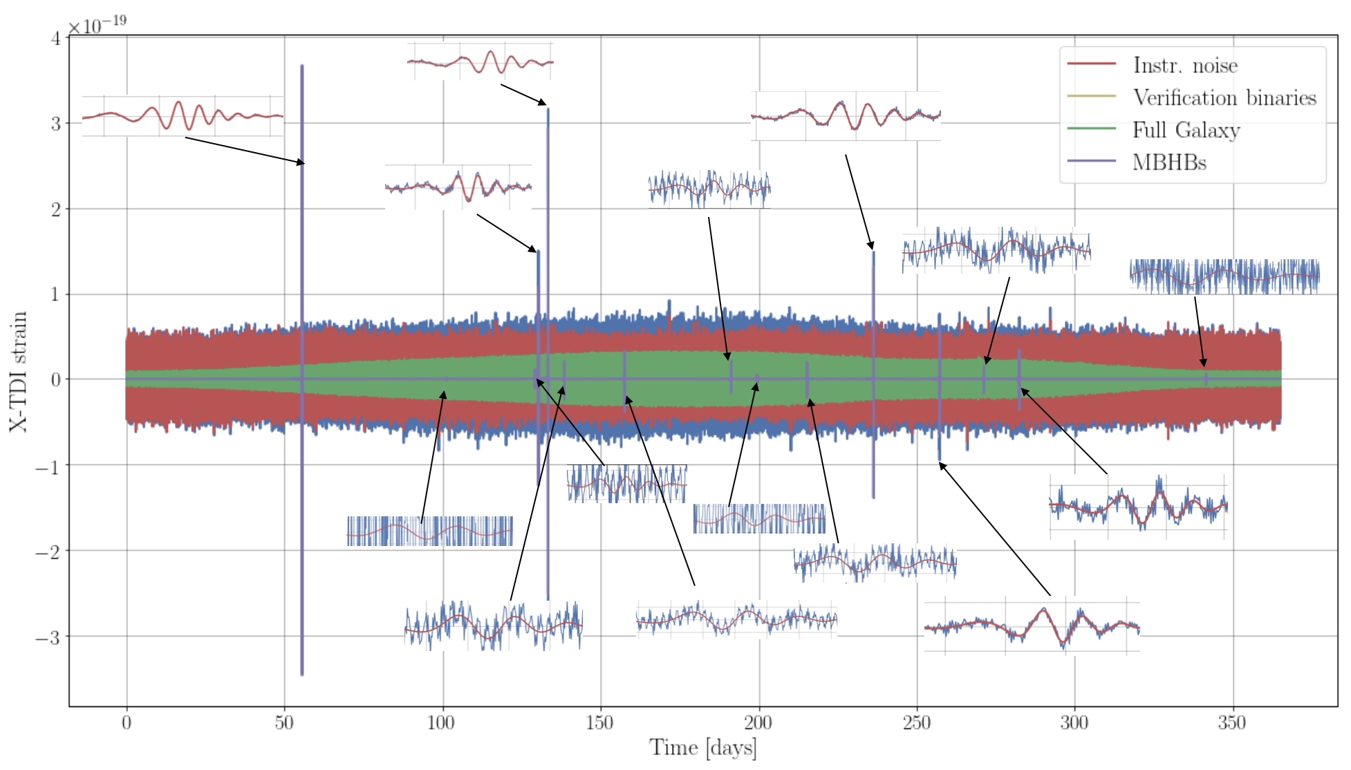
LIGO and Virgo have done it, so let's get LISA on the right path! MBHBs are represented with a frequency-domain inspiral-merger-ringdown phenomenological model (IMRPhenomD). The black holes are spinning, with spin vectors parallel to the orbital angular momentum. Waveforms contain only the dominant mode (which makes the challenge a bit harder); later we will issue datasets including higher-order modes from merging MBHBs. The training dataset contains 15 signals of various strength, sampled randomly from an astrophysical catalogue. These signals are shown in the time domain plot of the training dataset.

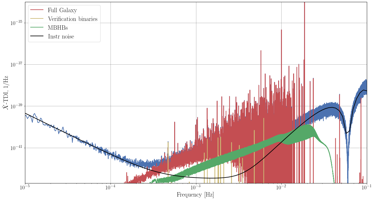
Generating 30 mln. Galactic binaries in time domain was a challenge and it took us few days on a large computing cluster. Let us see how long it will take to extract resolvable binaries (we expect more than 10,000 are detectable individually) and to estimate the stochastic GW foreground created by the remaining signals. Waveforms are idealized as monochromatic + first-derivative sinusoids; we have included both detached and interacting binaries, so the frequency derivative can be negative. These signals are in evidence in the frequency-domain plot of the training dataset.

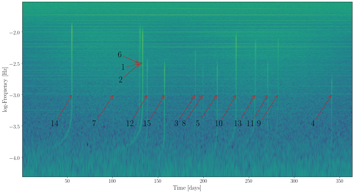
All sources (and especially the chirping massive black-hole tracks) are evident also in the time-domain map.

LDC2a. Blind data challenge.
The blind-challenge dataset was built in the same way and with the same waveform models as the training dataset. Noise level, signal parameters, and the number of sources were randomized. As suggested by the figures above, inspecting the data in the time, frequency, and time-frequency domains can provide valuable information.
